Rob Pike’s 5 rules of programming (and there is no rule six)

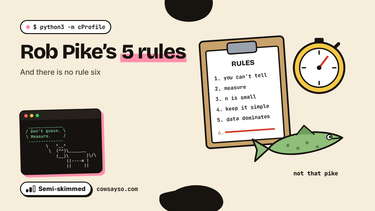
On 21 February 1989 a programmer at Bell Labs wrote some notes on how to program in C. Most of it is about C. But in the middle, under the heading “Complexity”, there are five short rules that have outlived the decade, the language and, quite possibly, the printer they were first printed on. Programmers still quote them in code reviews, usually right before ignoring them.

The programmer was Rob Pike. And no, not the fish. Although the fish is on the cover, because the cow has a sense of humour and no shame.

This is a semi-skimmed post: some code, nothing scary. Every example was really run, with Python 3.13 and Go 1.25, and the numbers are the real ones.

Who is Rob Pike

Rob Pike worked at Bell Labs on the Unix team, where he was one of the people behind Plan 9, Unix’s more ambitious and less famous successor, and the Blit graphical terminal. With Brian Kernighan he wrote two classic books, The Unix Programming Environment and The Practice of Programming.

He also has a habit of inventing things over dinner. By his own account, UTF-8, the encoding that today lets this very page show “è” and 🐄, was designed with Ken Thompson on a placemat in a New Jersey diner, one night around September 1992. Fifteen years later, on 21 September 2007, he, Thompson and Robert Griesemer started sketching a new language on a whiteboard at Google. It became public on 10 November 2009, and it’s called Go.

So when this man writes rules for programmers, it’s worth listening. Here they are, from “Notes on Programming in C”:

Rule 1. You can’t tell where a program is going to spend its time. Bottlenecks occur in surprising places, so don’t try to second guess and put in a speed hack until you’ve proven that’s where the bottleneck is.

Rule 2. Measure. Don’t tune for speed until you’ve measured, and even then don’t unless one part of the code overwhelms the rest.

Rule 3. Fancy algorithms are slow when n is small, and n is usually small. Fancy algorithms have big constants. Until you know that n is frequently going to be big, don’t get fancy. (Even if n does get big, use Rule 2 first.)

Rule 4. Fancy algorithms are buggier than simple ones, and they’re much harder to implement. Use simple algorithms as well as simple data structures.

Rule 5. Data dominates. If you’ve chosen the right data structures and organized things well, the algorithms will almost always be self-evident. Data structures, not algorithms, are central to programming.

And then, with a straight face: Rule 6. There is no Rule 6. Which sounds a lot like the Bruces of Monty Python, who in 1970 read out the rules of their Australian university, including the immortal “There is no rule six”. Pike doesn’t say. The cow likes to think so.

Rules 1 and 2: you can’t tell, so measure

The first two rules go together. Rule 1 says your intuition about performance is wrong. Rule 2 says what to do about it. Let’s test the first on ourselves. Here is a little program that processes 50,000 milkings: for each one it computes a “milk quality” with some very scientific, very scary maths (square roots, logarithms, π), and then counts how many different cows were milked.

import math, random

random.seed(42)
NAMES = ["Ercolina", "Pina", "Carolina", "Bianca", "Rosina", "Gelsomina"]


def milking_log(n):
    # n milkings: (cow name with a tag number, litres)
    return [(f"{random.choice(NAMES)}-{random.randrange(20000)}", random.uniform(5, 30)) for _ in range(n)]


def milk_quality(litres):
    # very scientific, very scary math
    return math.sqrt(litres) * math.log(litres + 1) / math.pi


def unique_cows(log):
    seen = []
    for name, _ in log:
        if name not in seen:
            seen.append(name)
    return seen


def report(log):
    quality = sum(milk_quality(litres) for _, litres in log)
    cows = unique_cows(log)
    return len(cows), round(quality, 1)


if __name__ == "__main__":
    print(report(milking_log(50_000)))

Before reading on: where do you think it spends its time? The maths, surely. All those square roots. Let’s run it:

$ time python3 herd.py
(40823, 190093.2)

real    0m8.301s
user    0m8.273s
sys     0m0.012s

Eight seconds to count some cows. Now, instead of guessing, we measure. Python ships with a profiler, cProfile, which tells you how much time each function takes:

$ python3 -m cProfile -s tottime herd.py
(40823, 190093.2)
         939959 function calls (939941 primitive calls) in 8.741 seconds

   Ordered by: internal time

   ncalls  tottime  percall  cumtime  percall filename:lineno(function)
        1    8.440    8.440    8.457    8.457 herd.py:17(unique_cows)
   100000    0.056    0.000    0.086    0.000 random.py:245(_randbelow_with_getrandbits)
        1    0.048    0.048    0.229    0.229 herd.py:7(milking_log)
    50000    0.030    0.000    0.083    0.000 random.py:345(choice)
    50000    0.024    0.000    0.073    0.000 random.py:295(randrange)
    50000    0.020    0.000    0.031    0.000 herd.py:12(milk_quality)
[...]

The scary maths, milk_quality, called 50,000 times: 0.03 seconds in total. The innocent little function that counts unique cows: 8.4 seconds, which is 97% of the whole run. The culprit is one harmless-looking line, if name not in seen: checking whether something is in a Python list means looking at every element, one by one. With 40,000 cows in the list, that’s a lot of looking.

That’s Rule 1 in action: the bottleneck was in the place nobody would have bet on. And Rule 2 is why we found it in ten seconds instead of spending a day optimising the square roots.

The famous phrase usually quoted next to these rules is “premature optimization is the root of all evil”. It comes from Donald Knuth, in a 1974 paper, and it’s often cut short: Knuth said we should forget about small efficiencies “about 97% of the time”, but not pass up our opportunities in “that critical 3%”. Rule 2 is the way to find that 3%. (Knuth later attributed the line to Tony Hoare, who said it wasn’t his. Even quotes have bottlenecks in surprising places.)

Rule 3: n is usually small

A “fancy” algorithm wins when there’s a lot of data, but it pays a fixed price every time: more setup, more memory, more bookkeeping. Pike calls them “big constants”. With little data, that fixed price is all you pay.

Let’s measure it, in Go, which seems only fair. We look for a cow in a herd in two ways: walking a slice from start to end, the dumbest thing that could work, or looking it up in a map, Go’s hash table.

// The simple way: walk the slice.
func findSlice(herd []string, name string) bool {
	for _, c := range herd {
		if c == name {
			return true
		}
	}
	return false
}

// The "proper" way: a map (Go's hash table).
//   found := set[name]

$ go test -bench .
goos: linux
goarch: amd64
pkg: herd
cpu: Intel Core Processor (Haswell, no TSX)
BenchmarkSlice5-4      	91375311	        12.06 ns/op
BenchmarkMap5-4        	100000000	        11.56 ns/op
BenchmarkSlice1000-4   	  656552	      1659 ns/op
BenchmarkMap1000-4     	79291477	        21.61 ns/op
PASS

With 5 cows, the dumb loop and the hash table are tied: 12 nanoseconds against 11.6. All the cleverness of hashing buys nothing. With 1,000 cows, the map is about 77 times faster. Both halves of Rule 3 in one table: when n is small, don’t get fancy; when n is big, the fancy structure earns its keep. And to know which case you’re in, see Rule 2.

Pike’s own example was harsher: “binary trees are always faster than splay trees for workaday problems”. Splay trees, published by Sleator and Tarjan in 1985, are an elegant structure with excellent theoretical guarantees. In 1989 they were a brand-new, elegant, fancy algorithm. Pike’s advice: for everyday work, the plain binary tree wins.

Rule 4: fancy algorithms are buggier

Even simple algorithms can hide bugs for years. Imagine the fancy ones. The most famous example is binary search, the algorithm every student writes in the first year. In 2006 Joshua Bloch, at Google, told the story of the binary search he had written for Java’s standard library: about nine years after it shipped, someone found it broken. The bug was in a line that looks perfect:

int mid = (low + high) / 2;

With arrays of more than about a billion elements (2³⁰), low + high exceeds the largest number an int can hold and wraps around to negative. We reproduced it in Go with 32-bit integers:

package main

import "fmt"

func main() {
	var low, high int32 = 1 << 30, 1<<31 - 1 // a herd of over a billion cows
	fmt.Println("broken:", (low+high)/2)
	fmt.Println("fixed: ", low+(high-low)/2)
}

$ go run main.go
broken: -536870912
fixed:  1610612735

A negative middle, which means reading outside the array. The same line was in the version of binary search published in Jon Bentley’s Programming Pearls, and Bentley himself noted that while the first binary search was published in 1946, the first one that works correctly for all values of n didn’t appear until 1962. Sixteen years, for an algorithm that fits on a napkin.

Ken Thompson, the man who wrote the first Unix, summed up Rule 4 in six words: “When in doubt, use brute force.”

Rule 5: data dominates

The last rule is the deepest, and Pike points to its source: Fred Brooks, The Mythical Man-Month, page 102. In Brooks’ words: “Show me your flowcharts and conceal your tables, and I shall continue to be mystified. Show me your tables, and I won’t usually need your flowcharts; they’ll be obvious.”

We’ve already seen Rule 5 at work. Remember the cow counter that took 8.4 seconds? The fix wasn’t a smarter algorithm. It was a different data structure: a set instead of a list.

def unique_cows(log):
    return set(name for name, _ in log)

$ time python3 herd_set.py
(40823, 190093.2)

real    0m0.097s
user    0m0.084s
sys     0m0.012s

From 8.3 seconds to a tenth of a second, about 85 times faster, and the function got shorter. With the right data structure, the algorithm is literally one line. That’s exactly what Rule 5 promises: choose the data well, and the code becomes self-evident.

It works for readability too, not only speed. Here’s the cow’s verdict system written the usual way, as a chain of ifs:

def verdict(action):
    if action == "deploy on friday":
        return "wrong"
    elif action == "measure first":
        return "right"
    elif action == "splay tree for 5 cows":
        return "wrong"
    elif action == "use a hash table":
        return "it depends"
    else:
        return "the cow is thinking"

And here it is with the data in charge: a table, and an algorithm that’s just “look it up”:

VERDICTS = {
    "deploy on friday":      "wrong",
    "measure first":         "right",
    "splay tree for 5 cows": "wrong",
    "use a hash table":      "it depends",
}

def verdict(action):
    return VERDICTS.get(action, "the cow is thinking")

print(verdict("measure first"))
print(verdict("rewrite it in rust"))

$ python3 verdict_table.py
right
the cow is thinking

Same behaviour. But now adding a verdict means adding a line of data, not a branch of logic; you can read all the rules at a glance, load them from a file, or test them in a loop. Pike also says that a handful of data structures cover almost all practical programs: arrays, linked lists, hash tables and binary trees, plus combinations of them.

So, what do we do with them?

The five rules fit in one sentence: don’t guess, measure; keep it simple until the data proves you wrong; and think about the data before the code. They don’t forbid optimising, or using clever algorithms. They ask you to do it for a reason you can show.

Thirty-five years later they still work, in C, in Python, in Go, and in languages that didn’t exist when they were written. Which is a good result for some notes written in 1989. Most of the code written that year doesn’t run anymore.

Moo. 🐄